Google Sheet Pivot Table Sort By Value

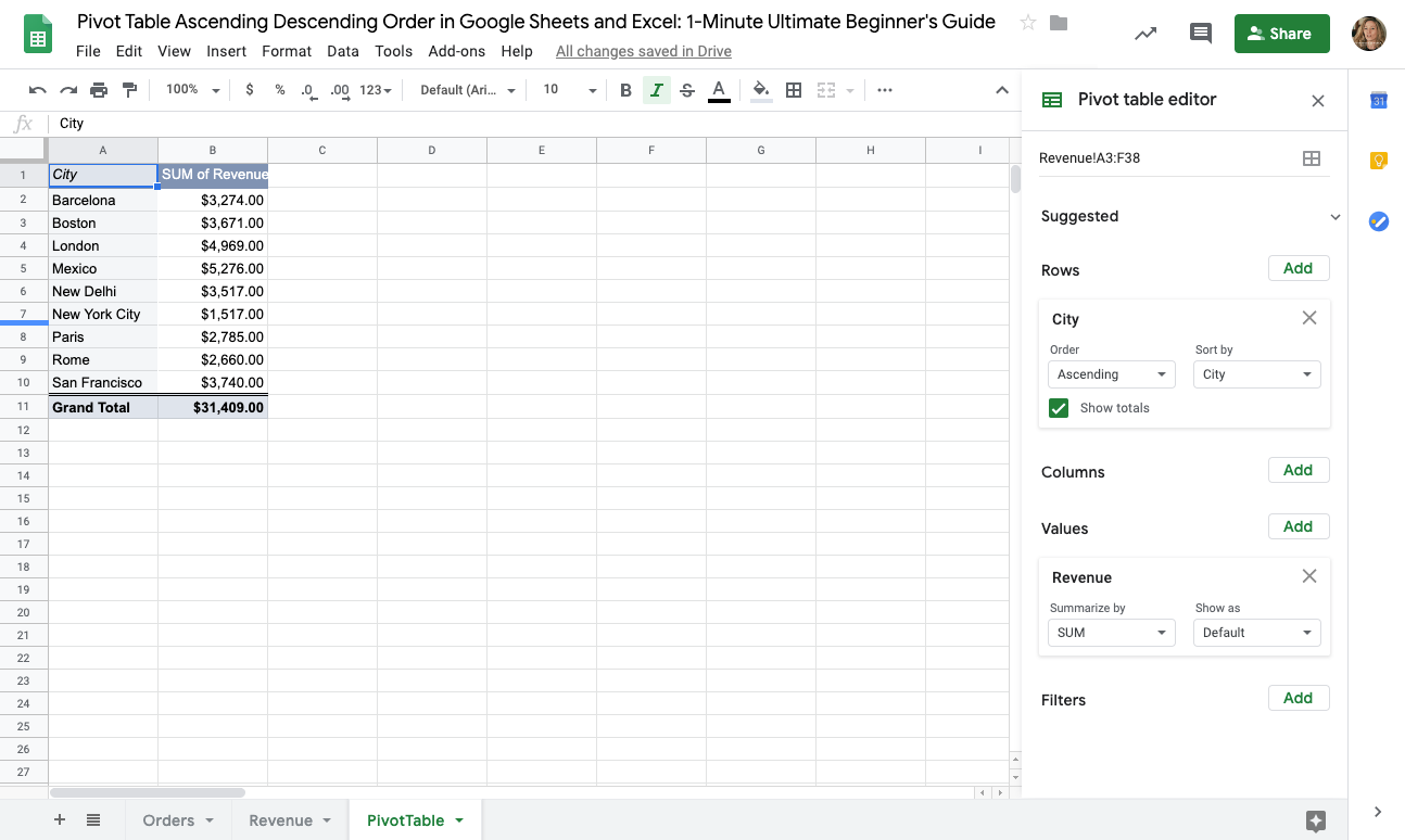
To show the totals of a row or column check show totals.

Google sheet pivot table sort by value. These filters can sort data in a different way than the built in pivot table filters and provide additional options for your data sets. At the heart of any pivot table are the rows columns and values. Select sort then choose either sort smallest to largest or sort largest to smallest. Click data create a filter.

If you are using this functionality at some point in time you may want to sort the grand total columns at the bottom of the pivot table report. To sort this data using the sort function in cell c2 enter the formula. In order to sort your spreadsheet data in a powerful and organized way we can add pivot tables to isolate specific data then slicers to further sort those tables. Group the days by day of week you can do this by week month day of the week or even units of time smaller than a day such as hour or minute.

On your computer open a spreadsheet in google sheets. Select a range of cells. Data pivot table. Google sheet has a wonderful function that makes the sorting easy as pie the sort function.

The best google sheets add ons. Choose which text or fill color to filter or sort by. On your computer open a spreadsheet in google sheets. Sort a2 b11 1 true.

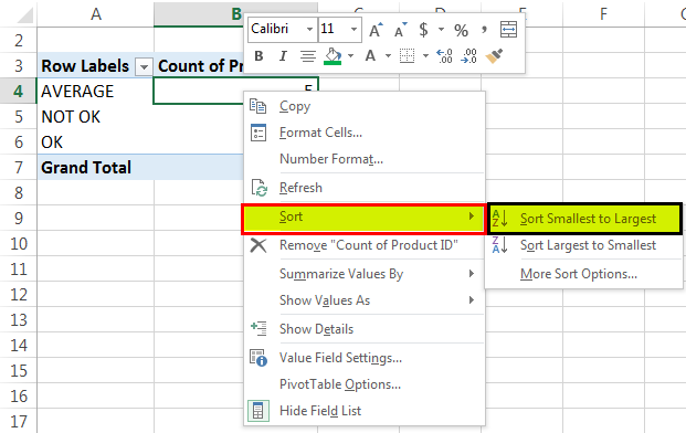
To sort the second column by value right click on a cell in second column s value field that is not a grand total. Use the cell e1 in the existing sheet to create the table. Next select any of the cells you want to use in your pivot. Fire up chrome and open a spreadsheet in google sheets.

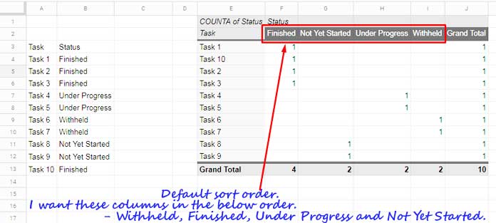
Columns add custom sort order the helper column. You can sort and order your data by pivot table row or column names or aggregated values. Columns add status. Rows columns and values.

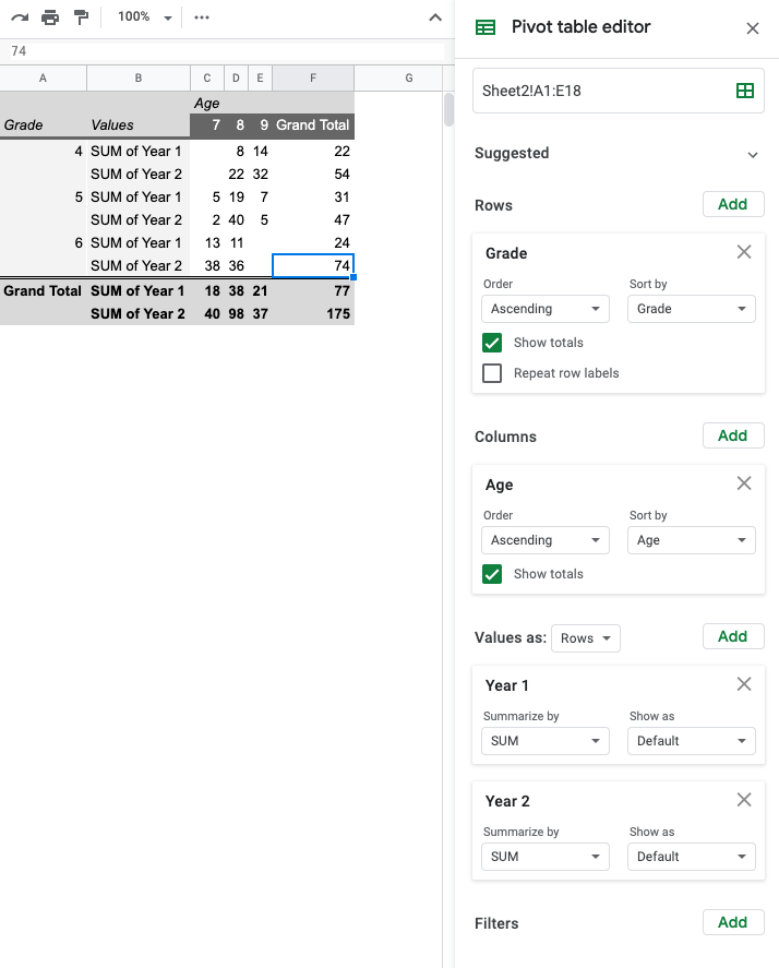
Under rows or columns click the arrow under order or sort by note. The settings inside the pivot editor. So let s take a look at building pivot tables in google sheets in more detail. When you create a pivot table from a table of data all of the columns from the dataset are available to use in your pivot tables.

Creating a pivot table from the information in the picture above displays a neatly formatted table with information from selected columns sorted by division. Sort data in google sheets using the sort function. Rows add task. The pivot table is quite useful for summarizing and reorganizing data in google sheets and as well as in other spreadsheets applications.

Click the pivot table. Suppose you have the data set as shown below. Change how your pivot table looks. Settings in pivot table editor to sort pivot table columns in the custom order.

Cells with the color you choose to sort by will move to the top of the range. To see filter options go to the top of the range and click filter. First select the range a3 c13.